- Introduction to time series analysis
Edward Ionides
1/05/2016
Licensed under the Creative Commons attribution-noncommercial license, http://creativecommons.org/licenses/by-nc/3.0/. Please share and remix noncommercially, mentioning its origin.
Objectives
Discuss some basic motivations for the topic of time series analysis.
Introduce some fundamental concepts for time series analysis: stationarity, autocorrelation, autoregressive models, moving average models, autoregressive-moving average (ARMA) models, state-space models.
Develop the computational framework for this course:
R and Rmarkdown for data analysis and reproducible documents
Source code sharing using git.
1.1 Overview
Time series data are, simply, data collected at many different times.
This is a common type of data! Observations at similar time points are often more similar than more distant observations.
This immediately forces us to think beyond the independent, identically distributed assumptions fundamental to much basic statistical theory and practice.
Time series dependence is an introduction to more complicated dependence structures: space, space/time, networks (social/economic/communication), …
1.1.1 Looking for trends and relationships in dependent data
The first half of this course focuses on:
Quantifying dependence in time series data.
Finding statistical arguments for the presence or absence of associations that are valid in situations with dependence.
Example questions: Does Michigan show evidence for global warming? Does Michigan follow global trends, or is there evidence for regional variation? What is a good prediction interval for weather in the next year or two?
1.1.2 Modeling and statistical inference for dynamic systems
The second half of this course focuses on:
Building models for dynamic systems, which may or may not be linear and Gaussian.
Using time series data to carry out statistical inference on these models.
Example questions: Can we develop a better model for understanding variability of financial markets (known in finance as volatility)? How do we assess our model and decide whether it is indeed an improvement?
1.2 A simple example: Winter in Michigan
Last winter was cold. Professor Shedden, who grew up in Michigan, said that it reminded him of how winters used to be. Let’s look at some data I downloaded from weather-warehouse.com and put in ann_arbor_weather.csv.
You can get this file from the course website (http://ionides.github.io/531w16).
Better, you can set up a local git repository that will give you an up-to-date copy of all the data, notes, code, homeworks and solutions for this course. More on this later.
y <- read.table(file="ann_arbor_weather.csv",header=1)Here, I’m using R Markdown to combine source code with text. This gives a nice way to generate statistical analysis that is
Reproducible,
Easily modified or extended.
These two properties are useful for developing your own statistical research projects. Also, they are useful for teaching and learning statistical methodology, since they make it easy for you to replicate and adapt analysis presented in class.
1.2.1 Question: How many of you already know R Markdown?
First, let’s get some basic idea what’s in our dataset. str summarizes the structure of the data:
str(y)## 'data.frame': 115 obs. of 12 variables:
## $ Year : int 1900 1901 1902 1903 1904 1905 1906 1907 1908 1909 ...
## $ Low : int -7 -7 -4 -7 -11 -3 11 -8 -8 -1 ...
## $ High : int 50 48 41 50 38 47 62 61 42 61 ...
## $ Hi_min : int 36 37 27 36 31 32 53 38 32 50 ...
## $ Lo_max : int 12 20 11 12 6 14 20 11 15 13 ...
## $ Avg_min : num 18 17 15 15.1 8.2 10.9 25.8 17.2 17.6 20 ...
## $ Avg_max : num 34.7 31.8 30.4 29.6 22.9 25.9 38.8 31.8 28.9 34.7 ...
## $ Mean : num 26.3 24.4 22.7 22.4 15.3 18.4 32.3 24.5 23.2 27.4 ...
## $ Precip : num 1.06 1.45 0.6 1.27 2.51 1.64 1.91 4.68 1.06 2.5 ...
## $ Snow : num 4 10.1 6 7.3 11 7.9 3.6 16.1 4.3 8.7 ...
## $ Hi_Pricip: num 0.28 0.4 0.25 0.4 0.67 0.84 0.43 1.27 0.63 1.27 ...
## $ Hi_Snow : num 1.1 3.2 2.5 3.2 2.1 2.5 2 5 1.3 7 ...Let’s focus on Low, which is the lowest temperature, in Fahrenheit, for each year.
There are practical reasons to understand the expected (i.e., mean) low temperature and the annual variation around this. Reasons to do this could be
Agriculture: can I grow ginseng in Ann Arbor?
Energy: assess the cost-effectiveness of installing extra home insulation.
Lifestyle: Should I move to Minneapolis, or Berlin, or Beijing?
Also, we could develop our analysis to look for evidence of climate change.
As statisticians, we want an uncertainty estimate. We want to know how reliable our estimate is, since it is based on only a limited amount of data.
Write the data as \(y^*_1,\dots,y^*_N\).
A basic estimate of the mean and standard deviation is \({\mu^*}= \frac{1}{N}\sum_{n=1}^Ny^*_n\) and \({\sigma^*}= \sqrt{\frac{1}{N-1}\sum_{n=1}^N(y^*_n-{\mu^*})^2}\), suggesting an approximate confidence interval for \(\mu\) of \({\mu^*}\pm 1.96{\sigma^*}/\sqrt{N}\),
1955 has missing data, coded as
NA, requiring a minor modification. So, we compute \({\mu_1^*}\) and \(SE_1={\sigma^*}/\sqrt{N}\) as
mu1 <- mean(y$Low,na.rm=TRUE)
se1 <- sd(y$Low,na.rm=TRUE)/sqrt(length(!is.na(y$Low)))
cat("mu1 =", mu1, ",  se1 =", se1, "\n")
## mu1 = -2.833333 , se1 = 0.68422751.2.2 Question: What are the assumptions behind the resulting confidence interval, \(-2.83 \pm 1.34\).
1.2.3 Question: When, in practice, is it reasonable to present this confidence interval? Is it reasonable here?
1.2.4 Question: How would you proceed?
1.2.5 Some data analysis
- The first rule of data analysis is to plot the data in as many ways as you can think of! For time series, we usually start with a time plot
plot(Low~Year,data=y,ty="l")
Another simple thing to do is to fit an autoregressive-moving average (ARMA) model.
- We’ll look at ARMA models in much more detail later in the course.
Let’s fit an ARMA model given by \[ Y_n = \mu + \alpha(Y_{n-1}-\mu) + \epsilon_n + \beta \epsilon_{n-1}.\] This has a one-lag autoregressive term, \(\alpha(y_{n-1}-\mu)\), and a one-lag moving average term, \(\beta \epsilon_{n-1}\). It is therefore called an ARMA(1,1) model. These lags give the model some time dependence.
If \(\alpha=\beta=0\), we get back to the basic independent model, \(Y_n = \mu + \epsilon_n\).
If \(\alpha=0\) we have a moving average model with one lag, MA(1).
If \(\beta=0\), we have an autoregressive model with one lag, AR(1).
We suppose that \(\epsilon_1\dots,\epsilon_N\) is an independent, identically distributed sequence. To be concrete, let’s suppose they are normally distributed with mean zero and variance \(\sigma^2\).
A note on notation:
In this course, capital Roman letters, e.g., \(X\), \(Y\), \(Z\), denote random variables. We may also use \(\epsilon\), \(\eta\), \(\xi\), \(\zeta\) for random noise processes. Thus, these symbols are used to build models.
We use lower case Roman letters (\(x\), \(y\), \(z\), \(\dots\)) to denote fixed numbers.
When fixed numbers are data or derived from data (i.e., statistics) we will often add an asterisk (\(x^*\), \(y^*\), \(\dots\)).
“We must be careful not to confuse data with the abstractions we use to analyze them.” (William James, 1842-1910).
Other Greek letters will usually be parameters, i.e., real numbers that form part of the model.
We can readily fit the ARMA(1,1) model by maximum likelihood,
arma11 <- arima(y$Low, order=c(1,0,1))We can see a summary of the fitted model, where \(\alpha\) is called ar1, \(\beta\) is called ma1, and \(\mu\) is called intercept.
arma11##
## Call:
## arima(x = y$Low, order = c(1, 0, 1))
##
## Coefficients:
## ar1 ma1 intercept
## 0.7992 -0.7533 -2.8479
## s.e. 0.3034 0.3295 0.8308
##
## sigma^2 estimated as 53.06: log likelihood = -388.14, aic = 784.27Write the ARMA(1,1) estimate of \(\mu\) and its standard error as \({\mu_2^*}\) and \(SE_2\). Some poking around is required to extract the bits of primary interest here.
names(arma11)## [1] "coef" "sigma2" "var.coef" "mask" "loglik"
## [6] "aic" "arma" "residuals" "call" "series"
## [11] "code" "n.cond" "nobs" "model"mu2 <- arma11$coef["intercept"]
se2 <- sqrt(arma11$var.coef["intercept","intercept"])
cat("mu2 =", mu2, ", se2 =", se2, "\n")## mu2 = -2.847949 , se2 = 0.8307836We see that the two estimates, \({\mu_1^*}=-2.83\) and \({\mu_2^*}=-2.85\), are close. However, \(SE_1=0.68\) is an underestimate of error, compared to the better estimate \(SE_2=0.83\). The naive standard error needs to be inflated by \(100(SE_2/SE_1-1)=\) 21.4 percent.
Exactly how the ARMA(1,1) model is fitted and the standard errors computed will be covered later.
We should do diagnostic analysis. The first thing to do is to look at the residuals. For an ARMA model, the residual \(r_n\) at time \(t_n\) is defined to be the difference between the data, \({y_n^*}\), and a one-step ahead prediction of \({y_n^*}\) based on \({y_{1:n-1}^*}\), written as \({y_n^{P\,*}}\). From the ARMA(1,1) definition, \[ Y_n = \mu + \alpha(Y_{n-1}-\mu) + \epsilon_n + \beta \epsilon_{n-1},\] a simple one-step-ahead predicted value corresponding to parameter estimates \({\mu^*}\) and \({\alpha^*}\) could be \[{y_n^{P\,*}} = {\mu^*} + {\alpha^*}({y_{n-1}^*}-{\mu^*}).\] A so-called residual time series, \(\{{r_n^*}\}\), is then given by \[ {r_n^*} = {y_n^*} - {y_n^{P\,*}}.\] In fact, R does something slightly more sophisticated.
plot(arma11$resid)
- We see that there seems to be some slow variation in the residuals, over a decadal time scale. However, the residuals are close to uncorrelated, as we can check by plotting their pairwise sample correlations at a range of lags. This is called the sample autocorrelation function, or sample ACF, which can be computed at each lag \(h\) for the residual time series \(\{r_n\}\) as \[ ACF(h) = \frac{\frac{1}{N}\sum_{n=1}^{N-h} {r_n^*} \, {r_{n+h}^*}} {\frac{1}{N}\sum_{n=1}^{N} {r_{n}^*}^2}.\] We will discuss the sample ACF at greater length later.
acf(arma11$resid,na.action=na.pass)
This shows not much sign of autocorrelation. In other words, fitting ARMA models is unlikely to be a good way to describe the slow variation present in the residuals of the ARMA(1,1) model.
There is probably some room for improvement over \(SE_2\), which might lead to a somewhat larger standard error estimate.
Although this is just a toy example, the issue of inadequate models giving poor statistical uncertainty estimates is a major concern whenever working with time series data.
Usually, omitted dependency in the model will give overconfident (too small) standard errors.
This leads to scientific reproducibility problems, where chance variation is too often assigned statistical significance.
It can also lead to improper pricing of risk in financial markets, a factor in the US financial crisis of 2007-2008.
1.3 Models dynamic systems: State-space models
Scientists and engineers often have equations in mind to describe a system they’re interested in.
Often, we have a model for how the state of a stochastic dynamic system evolves through time, and another model for how imperfect measurements on this system gives rise to a time series of observations.
This is called a state-space model.
The state models the quantities that we think determine how the system changes with time. However, these idealized state variables are not usually directly and perfectly measurable.
Statistical analysis of time series data on a system should be able to
Help scientists choose between rival hypotheses.
Estimate unknown parameters in the model equations.
We will look at examples from a wide range of scientific applications. The dynamic model may be linear or nonlinear, Gaussian or non-Gaussian. Here is an example from finance.
1.3.1 Fitting a model for volatility of a stock market index
Let \(\{y^*_n,n=1,\dots,N\}\) be the daily returns on a stock market index, such as the S&P 500.
Since the stock market is notoriously unpredictable, it is often unproductive to predict the mean of the returns and instead there is much emphasis on predicting the variability of the returns (known as the volatility).
Volatility is obviously related to the risk of financial investments.
Financial mathematicians have postulated the following model. We will not work on understanding it right now. The relevant point here is that investigators often find it useful to write down models for how a dynamic system progresses through time, and this gives rise to the time series analysis goals of estimating unknown parameters and assessing how successfully the fitted model describes the data.
\[ \begin{aligned} Y_n &= \exp\left\{\frac{H_n}{2}\right\} \epsilon_n, \\ H_n &= \mu_h(1-\phi) + \phi H_{n-1} \\ &\quad\quad + Y_{n-1}\sigma_\eta\sqrt{1-\phi^2}\tanh(G_{n-1}+\nu_n)\exp\left\{\frac{-H_n}{2}\right\} + \omega_n,\\ G_n &= G_{n-1}+\nu_n, \end{aligned} \]
\(\{\epsilon_n\}\) is an iid \(N(0,1)\) sequence, \(\{\nu_n\}\) is an iid \(N(0,\sigma_{\nu}^2)\) sequence, and \(\{\omega_n\}\) is an iid \(N(0,\sigma_\omega^2)\) sequence.
\(H_n\) represents the volatility at time \(t_n\). Volatility is unobserved; we only get to observe the return, \(Y_n\).
\(G_n\) is a slowly-varying process that regulates \(H_n\).
\(H_n\) has auto-regressive behavior and dependence on the previous return, \(Y_{n-1}\), as well as being driven by \(G_n\).
This is an example of a mechanistic model, where scientific or engineering considerations lead to a model of interest. Now there is data and a model of interest, it is time to recruit a statistician! (Statisticians can have roles to play in data collection and model development, as well.)
1.3.2 Relevant questions to be addressed using methodology covered later in the course
How can we get good estimates of the parameters, \(\mu_h\), \(\phi\), \(\sigma_\nu\), \(\sigma_\omega\), together with their uncertainties?
Does this model fit better than alternative models? So far as it does, what have we learned?
1.3.3 Outline of a solution
Likelihood-based inference for this partially observed stochastic dynamic system is possible, and enables addressing these questions (Bretó 2014).
Carrying out such an analysis is facilitated by recent advances in algorithms (Ionides et al. 2015).
The R package system and R markdown make state-of-the-art statistical analysis reproducible and extendable by Masters level statisticians! For example, with a modest amount of effort, you could run the code given in the online tutorial reproducing part of Bretó (2014). We will look more at these data and models later.
1.4 Internet repositories for collaboration and open-source research: git and github
Git is currently the dominant tool for managing, developing and sharing code within the computational sciences and industry. Github is the largest git-based internet repository, but others (such as bitbucket) also use git, and it can be useful to use git to build a local repository on your own computer.
This course will benefit directly from using git, since it provides a convenient way to manage the code, data, notes and other files involved in the course.
Also, you will be practicing a skill that will likely be useful for future work.
Our immediate goals are
Learn some ways to think about what a git repository is and how it works.
Go through the process of downloading a github repository, editing it, and uploading the changes.
This introduction uses material from Karl Broman’s practical and minimal git/github tutorial (kbroman.org/github_tutorial). A deeper, more technical tutorial is www.atlassian.com/git/tutorials.
This course will require only some basic familiarity with git, enough to download a project from github and to upload your own contribute the project.
1.4.1 Getting started with git and github
Get an account on github.
If you are on a Mac or Linux machine, git will likely be installed already. Otherwise, you can download and install it from git-scm.com/downloads.
Set up your local git installation with your user name and email. Open a terminal (or a git BASH window for Windows) and type:
$ git config --global user.name "Your name here"
$ git config --global user.email "your_email@example.com"
(Don’t type the $; that just indicates that you’re doing this at the command line.)
- Optional but recommended: set up secure password-less SSH communication to github, following the github instructions. If you run into difficulties, it may help to look at Roger Peng’s SSH help page.
1.4.2 Basic git concepts
repository. A representation of the current state of a collection of files, and its entire history of modifications.
commit. A commit is a change to one or many of the files in repository. The repository therefore consists of a directed graph of all previous commits.
branch. Multiple versions of the collection of files can exist simultaneously in the repository. These versions are called branches. Branches may represent new functionality, or a bug fix, or different versions of the code with slightly different goals.
Branches have names. A special name called master is reserved for the main development branch.
Branches can be created, deleted or merged.
Each new commit is assigned to a branch.
We now have the pieces in place to visualize the graph of a git repository. [Picture credit: hades.github.io]
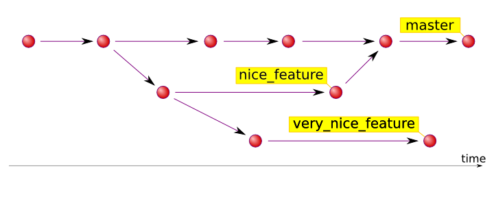

Take some time to identify the commits, branching events, and merging events on the graph.
Note that branch names actually are names for the most recent commit on that branch, known as the head of the branch.
1.4.3 An elementary task: cloning a remote repository
- In a suitable directory, type
git clone git@github.com:ionides/531w16You now have a local copy of the Stats 531 class materials.
The local repository remembers the address of the remote repository it was cloned from.
- You can pull any changes from the remote repository to your local repository using git pull.
$ git pull
Already up-to-date.
1.4.4 A workflow to contribute to the 531w16 github repository: Forking a project and making a pull request
We will follow a standard workflow for proposing a change to someone else’s github repository.
Forking is making your own github copy of a repository.
A pull request is a way to ask the owner of the repository to pull your changes back into their version.
The following steps guide you through a test example.
Click
forkat the top right-hand corner, and follow instructions to add a forked copy to your own github account. It should now show up in your account asmy_username/531w16.Clone a local copy of the forked repository to your machine, e.g.,
git clone git@github.com:my_username/531w16Equivalently, you can type
git clone https://github.com/my_username/531w16Move to the
531w16directory and edit the filehw0_signup.htmlto add your own name. You should use an ascii text editor, such as Emacs. Do not use Microsoft Word or any other word processing editor.It can be helpful to type
git statusregularly to check on the current state of the repository.
- Commit this change to your local version of the forked
531w16,
git add hw0_signup.html
git commit -m "sign up for my_name"
and see how the git status has changed. Another useful command for checking on the recent action in the repository is
git logType q to exit the listing of the log.
- Push this change to the forked
531w16on github:
git push- On the github web site for the
my_username/531w16fork, clickNew pull requestand follow instructions. When you have successfully placed your pull request, the owner of the forked repository (in this case, ionides@umich.edu) will be notified. I will then pull the modifications from your fork intoionides/531w16.
References
Bretó, C. 2014. On idiosyncratic stochasticity of financial leverage effects. Statistics & Probability Letters 91:20–26.
Ionides, E. L., D. Nguyen, Y. Atchadé, S. Stoev, and A. A. King. 2015. Inference for dynamic and latent variable models via iterated, perturbed Bayes maps. Proceedings of the National Academy of Sciences of the U.S.A. 112:719–724.